Over the course of the last month or so, YUSAG has begun using a model similar to our college football and college basketball models to analyze the NBA. Today I wanted to explain a couple of the mathematical points that go into the model and some of our predictions. To see the R code that we use to make our NBA models, click here! To see the latest NBA Power Rankings click here! To see the latest NBA Playoff predictions, click here! Follow @YUSAG_NBA on twitter for the latest updates!
Model 1: NBA Power Rankings (Linear Regression)
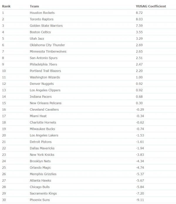
Our first NBA model generates the YUSAG Coefficients, which we use to find the relative point differential between two teams. Subtracting the two values gives you a predicted score differential if the two teams were to play at a neutral location.
An example of these ratings from March 17 2018 is shown here.
The question becomes, how do we produce these YUSAG Coefficients for each team, and how does the score prediction account for someone being the home team? Luckily, we can kill both of these birds with one stone: a linear model!
Most people think of linear models in terms of 1 predicting parameter because this is the easiest way to visualize it. When you fit a trend or best fit line on excel, you’re finding the slope and intercept parameter that minimize the term:
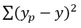
were yp shows the predicted y.
In our model, we are doing the same thing: minimizing the sum of the squared differences between the predicted score for an NBA game and an actual NBA game. yp corresponds to the predicted score differential, while y corresponds to the true score differential. The predictor variables we use are a team, their opponent, and the location the game is being played in. When we fit our model using the lm() function in R, we are finding the combination of 31 different coefficients (1 for each team and 1 for home field advantage) that minimize the sum of the squared errors. The formula we use for the predicted score at a given team’s home court is
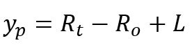
here Rt and Ro represent the YUSAG Coefficients for the team and their opponent. The location will either add or subtract a little bonus depending on whether the team is home or away. This bonus should be equal and opposite.
When we fit our model (find the set of 31 coefficients that minimizes the error), we see something that looks like this.
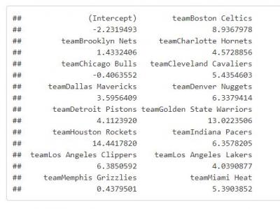
The result of our model fit is then 30 numbers, each corresponding to a team, and a single number that corresponds to the bonus given to the home team. We’ve found this to be ~2.1 points. Think about how many NBA games are decided by 4 or less points and you’ll see why home field advantage is such a big deal! After cleaning up our results, we have the final gridded YUSAG coefficients. Check out the latest values here!
Model 2: Win Probability (Logistic Regression)
The next goal of our model is to turn our predicted score differential into a win probability. To do this, we will fit a logistic function. If you took intro bio at some point, you might remember this as the population growth function. It looks something like this
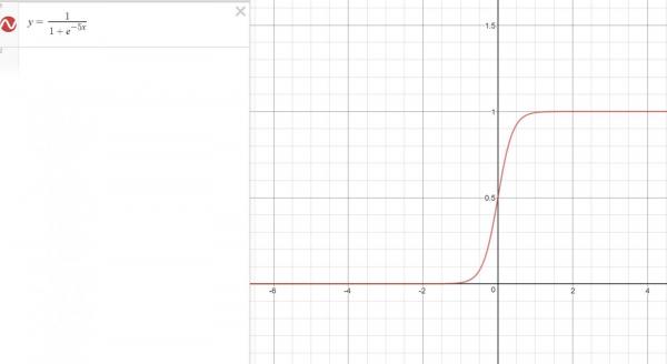
There is a carrying capacity which is the numerator of the equation. Y will go from 0 to this carrying capacity as x goes from -infinity to infinity. This is the perfect function to simulate win probability. As our predicted score differential increases, the win probability should approach, but never reach 1. If we are predicting a tossup, with score differential right around 0, it makes sense that the win probability is around .5.
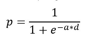
To fit this function for our NBA model, we tell R to look at all our predicted score differentials, then look at whether or not the team actually won. We start out with the equation for win probability below where d is the predicted score differential and the parameter we are changing is a, then find the a that results in the smallest sum of the squared errors by fitting the best logistic function to our data.
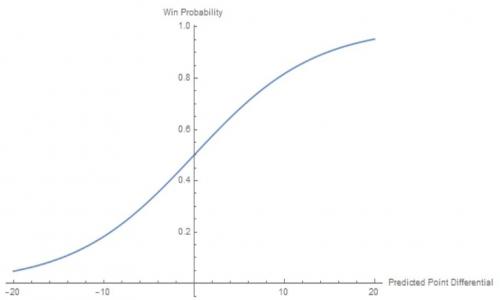
For the most part, when we fit the parameter a this gives us a value between .14 and .16. The resulting fit function looks something like this
This function helps us to predictjust how likely it is for our predictions to be right. For example, take a look at this plot below, where we have filled in our function with games taking place throughout the 2017-2018 season.
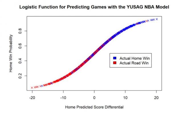
As one might expect, the larger home predicted point differentials correspond far more often, but not always, in actual home victories.
Simulations: Predicting End of the Season Standings
Once we have a model that gives us the predicted point differential and win probability for a given game, we can predict games that are happening today and tomorrow. Follow @YUSAG_NBA on twitter where we post our daily updates. Once we can do this, though, why can’t we simulate an entire season? How about finding the probability that a team will make the playoffs this season, or something similar?
Actually, calculating the probability that a given team will make the playoffs requires far more calculations than any of us would want to do on our own. It turns out there’s an easier way to get an approximation. When you flip a coin, there’s a .5 chance that the result will be heads. If you flip a coin twice though, you won’t necessarily get 1 head and 1 tail. As you flip a coin a lot of times, however, you’ll eventually notice that the fraction of heads will approach and eventually be very close to 1/2 our expected value. The same can be done here. If we simulate many NBA seasons and count how many times the Clippers make the playoffs, we can find a value pretty close to the actual probability that they’ll make the playoffs.
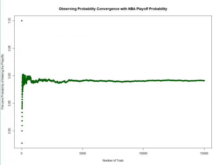
In order to simulate one season, we can think of it as flipping “g” number of coins, where g is the number of games we are simulating. Instead of p = .5, these are weighted coins. To flip a weighted coin, for example one with p = .8, we generate a random number between 0 and 1. If the random number is less than p, it’s a success. If it’s greater than p, it’s a failure. In this case, a win or a loss. We can flip a coin for each game remaining in the season, then see who has the number one seed, who has the best odds in the lottery, and who just missed out on the playoffs. When we repeat this over N simulated seasons, we can start to get an idea of some probabilities. For our model, I like to use 15,000 simulations. The plot below (which shows the Pelicans playoff chances for the 2017-2018 season) shows how the probability converges to a value as N gets larger.
Check out the latest playoff probabilities here, and be the lookout for YUSAG NBA Finals probabilities coming soon!